
This post offers an estimate of long term marginal CO2 emissions from electric power generation for use in determining the life cycle environmental benefits of heat pump conversions happening in the mid 2020s. This post was originally based on the 2021 Avoided Energy Supply Cost study. The 2024 Avoided Energy Supply cost study leads to an estimate of over 308 kgCO2/MWH in winter. See 2024 update at end of post. Using a winter value makes most sense for heat pump computations. This estimate is specific to the New England region.
As heat pumps become more common in New England homes, they will increase demand for electricity. How will that demand be served — by what mix of wind, solar, nuclear, hydro, oil, or natural gas? How will carbon emissions from electricity generation change as a result?
The answers appear fairly clear: Within the policy and economic landscape that we have today in New England, we can expect to lower our total emissions by building renewable power sources. However, to the extent we add significant electricity demand from heat pumps and electric vehicles on top of our existing demand, that additional demand will mostly fire up natural gas power generators.
This post analyzes and reconciles grid projections for New England from two well-funded and well-executed modeling exercises, both of which are designed to support public policy analysis and business decisions:
- The New England regional Avoided Energy Supply Cost Study (AESC 2021). The AESC is sponsored by the AESC Study Group, “a group representing all of the major electric and gas utilities in New England as well as efficiency program administrators, energy offices, regulators, and advocates.” It has been repeated every few years since 2007. It serves as the basis for benefit-cost computations in Mass Save program planning.
- The National Renewable Energy Laboratory’s Cambium Model, updated through September 2022. Cambium is actually a collection of output from ReEDS, a model of the national power grid funded by the Department of Energy. It was first published in 2020 and is updated annually. It has been used to make national estimates of heat pump green house gas emissions.
These two models report strikingly different projections for marginal emission rates in New England, with Cambium offering much lower estimates. However, review of the details of the models’ outputs and methodology clarify that the models project similar physical futures for New England’s power grid and similar marginal emissions rates from New England power generation. The authors of both models agree that Cambium’s low estimate of marginal emissions rate is due to its application of a national default assumption about the regional markets for Renewable Energy Credits, a default assumption that is not expected to be true in New England (and which, even if it became true, would not necessarily alter the physical marginal emissions from New England power generation that would be induced by increased electrical demand).
Concepts
ISO New England: Massachusetts is interconnected with New England states. ISO New England is the balancing authority that directs power generators to turn power on and off to meet electric demand. ISO-NE is also the primary source for data about power generation in New England.
Emissions: Fossil fuel power plants emit multiple pollutants — of most concern are carbon dioxide, sulfur dioxide, nitrogen oxides and particulates. Emissions are expressed as weight of pollutant (pounds/tons or kilograms/metric-tons).
Average emissions rate: Total emissions divided by total energy generated over some period of time. The units of average emissions rates are weight per amount of electrical energy, for example “pounds CO2 per kilowatt hour” (lbsCO2/kwh) or “metric tons CO2 per megawatt hour” (MTCO2/mwh) or “kilograms CO2 per megawatt hour” (kgCO2/mwh), etc.
Marginal emissions rate: The emissions that will be added as a result of added demand divided by the amount of added demand — expressed in the same units as average emissions rate (for example kgCO2/kwh). The marginal rate of emissions could be zero if the added demand is satisfied by hydro, but will be approximately .97 pounds per kilowatt hour (which is the same as 452kg/MWH) if the added demand is satisfied by firing a natural gas plant. Grid power sources and the resulting marginal rate of emissions vary by time of day and season. See ISO New England’s more precise definition of marginal emissions rate.
Long-run marginal emissions rate (LRMER) vs short run marginal emissions rate: The marginal emissions rate could be evaluated over a short period or a long period. The short run emissions rate is a function of what generating resources are dispatched as opposed to what resources are added or subtracted from the grid. That is in contrast to the long run rate. As the National Renewable Energy Laboratory explains: “The LRMER is an estimate of the rate of emissions that would be either induced or avoided by a long-term (i.e., more than several years) change in electrical demand. It incorporates both the projected changes to the electric grid, as well as the potential for an incremental change in electrical demand to influence the structural evolution of the grid (i.e., the building and retiring of capital assets, such as generators and transmission lines). It is therefore distinct from the more-commonly-known short-run marginal, which treats grid assets as fixed.”
Average vs. marginal emissions rates: Average emissions rates reflect all of the power generation resources on the grid. Marginal emissions rates (whether short or long term) reflect the power generation resources that might be added as a result of additional demand. In New England today, we have some green power resources, but the marginal resources that can be dispatched as needed to meet additional demand are mostly fossil-fuel resources, so the marginal emissions rate is usually higher than the average emissions rate. In some conversations, the choice between the two measures takes on a philosophical flavor — why should heat pumps or electric vehicles be evaluated at the higher marginal rate instead of being averaged into the normal base (which is comprised of lighting, hot water heating, office equipment, etc.)? Indeed, over time heat-pumps and EVs should and will be thought of as part of the base. However, some public policy measures directly increase or decrease electrical demand. For example, incentives to replace fossil fuels heat with heat pumps increase electrical demand; incentives to upgrade inefficient air conditioners reduce electrical demand. To evaluate those incentives, one wants to know how they will affect overall emissions, including electric generation emissions. For this purpose, the relevant metric is the LRMER, the long term marginal emissions rate. The Avoided Energy Supply Cost Study (AESC) and the Cambium Model are both purpose-built to supply LRMER estimates to support policy evaluation.
Busbar vs end use (this is a fine point): The energy denominator in an emissions rate can be measured at the busbar (i.e, the point of generation), or at the point of end use. The latter metric reflects transmission and distribution losses and so results in a slightly higher value for any emissions rate. In all charts in this post, MERs are reported using energy at the busbar in the denominator. The only exceptions are the Cambium-2020 LRMERs in the 2021 and 2023 comparisons; Cambium-2020 only published enduse LRMER.
Comparing marginal emissions rate projections
Cambium produces much lower marginal emission rate projections than the AESC. Cambium’s projections are also much lower than actual measured marginal emission rates in 2021.
Annually, ISO New England publishes an Air Emissions Report on power generation in the region which includes actual short run marginal emissions rates. The most recent available year of that study is 2021. The most recent AESC was published in early 2021 and the 2020 version of Cambium was published in August 2021. The chart below compares their projected long-run rates for the full year of 2021 with the ISO actual short run results. The AESC projection for full year 2021 was very close to the measured actual result for 2021. The Cambium projections are more than 60% below the measured actual result in all three scenarios. Note that the projections from Cambium do not sort as one might expect from the low-mid-high scenario naming.
Comparing the long-run models to the actual results is not entirely fair because short run rates reflect dispatching practices, not grid changes over time in response to load. Additionally, the long run models reduce reported emissions by Renewable Energy Credit purchases, while the ISO report is entirely physical. However, over a one or two year period, grid change is unlikely — in the AESC model, the grid is actually assumed to be fixed for the first three years — so short run marginal rates should be close to long run marginal rates unless RECs play a big role (which, as further discussed below, turns out to be part of the story).
Comparing Cambium and AESC Projected to Actual for New England Region 2021
| New England Marginal Emission Rate Source | Marginal Emissions Rate in 2021 (kgCO2/mwh) |
| ISO 2021 Air Emissions Report, Actual Short Run (Load Weighted Marginal Emissions, Table 5-5) | 343 |
| Avoided Energy Supply Cost Study 2021* LRMER Projected | 354 |
| Cambium 2020 LRMER Workbook** LRMER Projected Mid-Case Scenario | 135 |
| Cambium 2020 LRMER Workbook** LRMER Projected Low Renewable Cost Scenario | 103 |
| Cambium 2020 LRMER Workbook** LRMER Projected High Renewable Cost Scenario | 116 |
** LRMER Spreadsheet with start year investment of 2021 and duration 1 year. Taking average of 24 hour-of-day results. Note that the LRMER spreadsheet assumes marginal emissions in 2021 are the same as in 2022 and uses the modeled 2022 value.
The 2022 version of the Cambium model was last updated in January 2023 and includes state and federal policy revisions through Fall 2022. As the chart below shows, the Cambium-2022 marginal emission rate projections for 2023 run much higher than the Cambium-2020 projections for 2023. It is unclear what changed assumptions or model revisions drive the Cambium-2022 projections so far above the Cambium-2020 projections. The most notable intervening event was the passage of the landmark federal Inflation Reduction Act, which intuitively would have lowered projections.
Although Cambium-2022 offers higher projections than Cambium-2020, the Cambium-2022 projections for 2023 still come in 18% below the actual short run results shown in the preceding table for 2021. The AESC projected a slightly higher rate for 2023 than for 2021.
Cambium and AESC Projections for New England Region 2023
| New England Marginal Emission Rate Projection Source | 2023 Marginal Emissions Rate (kgCO2/mwh) as projected in 2021 | 2023 Marginal Emissions Rate (kgCO2/mwh) as projected in 2023 |
| Avoided Energy Supply Cost Study 2021* | 358 | updated projection not available |
| Cambium 2020 and 2022 LRMER Workbooks** Mid-Case Scenario | 71 | 280 |
| Cambium 2020 and 2022 LRMER Workbooks** Low Renewable Cost Scenario | 85 | 277 |
| Cambium 2020 and 2022 LRMER Workbooks** High Renewable Cost Scenario | 79 | 270 |
** LRMER workbooks from Cambium-2020 and Cambium-2022 with start investment of 2023 and period of one year. Taking average of 24 hour-of-day results in 2020 version. In the Cambium 2022 version, one has additional options. Those were set to include only combustion emissions, so excluding gas leaks during production. AESC does not reflect gas leaks. Note that both Cambium LRMER spreadsheets assume marginal emissions in 2023 are the same as in 2024 and uses the modeled 2024 value.
Looking longer term, AESC and Cambium-22 diverge further. AESC forecasts little drop in marginal emissions through 2035. In the ASEC, although renewables increase their generation share, gas power remains frequently at the margin and LRMER remains at 326. By contrast, there is no Cambium-22 scenario with an LRMER over 181 in 2035. The difference between AESC and Cambium-22 is much wider than the differences among Cambium-22 scenarios.
Comparing ASEC and Cambium 2022 projections for 2035
| New England Marginal Emission Rate Source | Marginal Emissions Rate in 2035 (kgCO2/mwh) |
| Avoided Energy Supply Cost Study (AESC)* | 326 |
| Cambium 2022 LRMER Workbook** Mid-Case Scenario | 173 |
| Cambium 2022 LRMER Workbook** Low Renewable Cost Scenario | 135 |
| Cambium 2022 LRMER Workbook** High Renewable Cost Scenario | 162 |
| Cambium 2022 LRMER Workbook** Electrification Scenario | 164 |
| Cambium 2022 LRMER Workbook** Low Natural Gas Price Scenario | 181 |
** LRMER spreadsheet with start investment of 2035 and period of one year; including only combustion emissions, so excluding emissions during production from leaks, etc. Viewing emissions from an end-user perspective, so including transmission losses. AESC does not consider leaks.
Comparing projections of grid development
One can gain some insight into the low LRMERs projected by Cambium-22 by exploring the actual changes in the generation sources that the model projects in different scenarios. Scenario details may be downloaded from the Cambium Scenario Viewer. A comparison of scenarios offers an alternative Cambium-22-based computation for LRMER that is very consistent with AESC.
The Cambium-22 Electrification scenario is identical to the Cambium-22 Mid-Case scenario except that it simulates a higher rate of electrification, positing a higher annual demand growth rate of 1.99%. The model projections in these two closely related scenarios show that in response to an increased electrification load, the Cambium-22 model adds mostly natural gas a generating resource in 2035.
Comparing Cambium-22 Scenarios for 2035 — Mid-Case vs Electrification
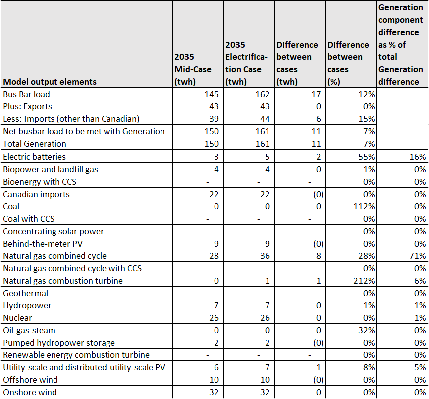
The Cambium output also includes total emissions from generation, allowing a computation of Long Run Marginal Emissions Rate for 2035 as the difference in emissions from the two scenarios divided by the difference in generation from the two scenarios. Unsurprisingly since natural gas dominates as the marginal source of power, marginal emissions computed from Cambium-22 through this approach are surprisingly close to marginal emissions in the ASEC — 305 vs. 326 kgCO2e/Mwh. Note that the Cambium-22 output does include Canadian hydro, but does not allow an imputation of the GHG impact from other imports.
Computation of Long Term Marginal Emissions Rate in 2035 from Cambium-22 Scenario Comparison
| Total Combustion Emissions from generation in Mid Case (MTCO2) | 11,071,463 |
| Total Combustion Emissions from generation in Electrification Case (MTCO2) | 14,406,422 |
| Incremental Emissions (MTCO2) | 3,334,959 |
| Incremental Generation (MWH) | 10,946,430 |
| Long Run Marginal Emissions Rate from Generation (kgCO2/Mwh) at the bus bar | 305 |
| Long Run Marginal Emissions Rate from Generation (kgCO2/Mwh) after distribution losses | 322 |
| Memo: Long Run Marginal Emissions Rate for 2035 from AESC* | 326 |
According to Cambium lead author, Pieter Gagnon, the basic mechanism for determining marginal emissions in Cambium is to increase load in a given scenario by 5% and see how much additional emissions the model projects. Using the scenario comparison above, we have increased the Cambium Mid-Case load by modestly more (12%) and derived a very different Cambium-based estimate of LRMER, one much more consistent with AESC.
Reconciling Cambium and ASEC
At the physical level, both AESC and Cambium-22 project substantial renewable builds in New England, yet they both project mostly gas-powered generation as the further response to load increases above baseline growth. However, both models not only make physical projections, but also project the trading of Renewable Energy Credits to comply with state Renewable Portfolio Standards. Reported LRMERs in both models reflect physical emissions as adjusted to reflect Renewable Energy Credits transactions with regions adjacent and connected to the New England Grid. As explained below, there is an important difference in how the models treat Renewable Energy Credits which explains the difference in reported LRMERs.
Renewable Portfolio Standards require utilities to purchase a defined share of their energy needs from renewable energy sources. To the extent that a utility is unable to directly purchase renewable energy to meet the standard, the utility can purchase credit for renewable energy either from another utility that is exceeding its RPS standard or from a non-utility renewable producer (like a homeowner with roof-top solar). New England utilities can purchase RECs from qualifying generators within New England or in regions adjacent to and connected with the New England power grid. See page 145ff. of the AESC for details of RPS policies of New England states.
It could happen that in a given year in a given state, the RPS would not actually be “binding.” This would happen if other state procurement policies and incentives lead to expected renewable build-outs more than sufficient to cover RPS obligations. The AESC offers this example:
[C]onsider a hypothetical where utilities in a state with 20 TWh [of annual load] are (a) required to purchase 12 TWh of renewable resources in any given year, and (b) the state also has an RPS wherein utilities must purchase and retire RECs equivalent to 50 percent of their electricity sales (10 TWh). In this hypothetical, the state’s RPS policy is exceeded by 2 TWh, meaning that changes to load (short of increasing load by 2 TWh) will not have an impact on the quantity of renewables purchased by that state.
AESC at page 191.
AESC’s modeling team conducted extensive New England specific analysis (see Chapters 7 and 8 of the AESC) of how REC requirements would interact with other renewable energy policies. See AESC at pages 154-5 for a list of considered non-RPS policies and incentives. Their conclusion is that across New England, RPS policies are not likely to become “binding” through 2035.
Based on our renewable energy market fundamentals analysis, we anticipate an RPS compliance surplus in each state, in each [scenario], and in each study year. REC supply and demand are expected to be closest to equilibrium during the first three years of the study period. During this time, while current-year REC supply may trail current-year demand in one or more years, RPS-obligated entities currently hold large ‘bank balances’ (which refers to excess RPS compliance that LSEs collectively already have at their disposal) which can be used to fulfill RPS obligations and therefore provide a clear signal that no incremental renewable energy builds are required. In the middle and later years of the study period, regional REC surpluses of up to 5,600 GWh per year are expected. . . .
AESC at page 191-2.
In other words, because regional REC surpluses are expected throughout the study period—obviating the need for renewable energy builds beyond policy-mandated supply—in all [scenarios], any quantity of demand-side measure deployed (whether it increases or decreases demand) is unlikely to affect the quantity of renewables built.
Cambium-22, being a national model, cannot do an extensive regional REC market analysis and effectively defaults to an assumption that marginal increases in non-renewable power generation would require marginal REC purchases. In computing an LRMER for a scenario, Cambium reruns its national model of grid response for that scenario but increases the demand assumption. It then looks at how the national generation mix changes and allocates the change to each state. It then applies state RPS policies to the generation change for each state — so implicitly assuming that if the change in generation is primarily fossil, then RECS will be purchased to offset make the change compliant on its own, without considering the possibility that the change might simply take up an existing surplus of RECs within the state. The model decreases state emissions by RECs purchases and increases emissions by REC sales. See Cambium-22 documentation, section 6.4, especially at pages 49-50. Thus, since New England modeled emissions at the margin in 2035 are from natural gas, Cambium-22 decreases them with out-of-region REC purchases. For the reasons explained above, those out-of-region REC purchases would not actually be necessary based on the surplus of RECs within New England caused by non-RPS policies. In recent conversations and email exchanges, both model authors (Pieter Gagnon for Cambium and Pat Knight for AESC) confirm that the Cambium REC methodology overstates REC purchases and understates marginal emissions in New England and accounts for most of the difference between ASEC and Cambium-22.
While the Cambium-22 New England LRMER is understated as a result of Cambium’s currently not-applicable assumption that RPS standards would be binding in New England, it does offer a useful model of a policy scenario in which RPS standards in New England are raised to binding levels. Even in that scenario, Cambium does not predict new renewable generation capacity in response to increased demand. In other words, if New England states were to increase RPS requirements to the point that they did become binding, the consequence would likely be either to increase the purchase of RECs from outside New England or to force utilities to make alternative compliance payments, as opposed to stimulating additional renewable builds within New England. The latter is likely if neighboring energy markets also adopt more aggressive RPS requirements.
Note on an additional modeling exercise
The Massachusetts Secretary of Environmental Affairs is charged with developing a roadmap to net zero emissions by 2050. As part of developing that roadmap, the Secretary retained consultants to evaluate different possible scenarios or pathways towards that goal. That planning exercise touches a wide range of issues and the published documentation of the modeling is at a more general level than the very detailed documentation for the ASEC and Cambium. However, the planning documents include a workbook which includes data on total electric generation under the alternative scenarios.
From that workbook, we can derive a 2040 scenario comparison similar to the 2035 comparison done above for Cambium. As in the Cambium 2035 comparison, an increase in modeled electrical load leads to an increase in gas generation and imports, but no additional renewable generation. There are many more variables moving around in these scenarios than in Cambium, but the scenario comparison nonetheless offers an additional crude confirmation of how gas remains at the margin even in scenarios involving large renewable builds. Note that, for simplicity, the table below combines wind and solar and nets out the use of power for electrolysis which is a prominent feature of the “Clean Fuels” Scenario; if one does not net out electrolysis, renewables appear to actually drop as the model adds electrical load.
Comparison of lowest and highest electrification scenarios in MA Clean Energy Climate Plan for 2040
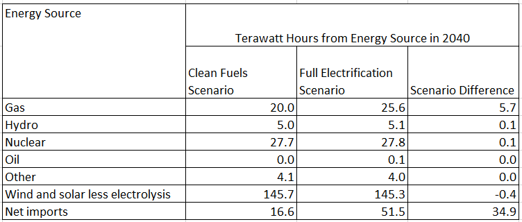
By 2040 in the full electrification scenario, the EoEEA model predicts that the New England grid would shift from a summer peak to a winter peak. The model forecasts a peak New England electrical demand of 58 Gigawatts (GW) at 7AM on a January morning. At that time of day in winter, solar would be unavailable. The total installed wind capacity is modeled at 26 (GW) — insufficient enough to cover half the load (and the wind might not be blowing); nuclear provides only another 3.3GW. A combination of cost-effectiveness and the need for reliable peak power contribute to the continued use of gas. See additional discussion of the EoEEA model here.
Conclusion
In the New England market, both the Avoided Energy Supply Cost study and Cambium-22 indicate that marginal increases in electrification will mostly be served by natural gas generators well into the next decade. Apparent differences in LRMER computations derive not from differences in physical projections, but from a national assumption about REC purchases which is built into Cambium-22 which is not applicable in the New England Market. Accordingly, Cambium modeling offers no reason to doubt the regionally developed LRMER projections from the AESC which continue to run above 300 kgCO2/mwh well into the next decade due to the persistence of natural gas as the marginal generation source even as renewables expand. EoEEA modeling is not to the contrary. For my own analysis of heat pump options, since the number is well founded and apparently in the right ball park, I will use the ASEC long run marginal costs from 2023 through 2035 without discounting: 342 kgCO2/mwh. Of course, major economic or policy shifts could alter expected emissions.
2024 Update
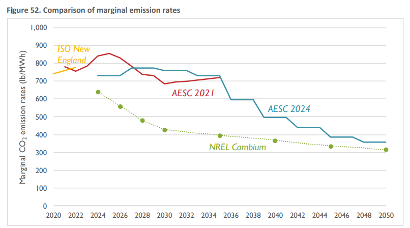
The 2024 Avoided Energy Supply Cost Study was released in February 2024. The study updates and extends projections for long run marginal emissions. As shown in the figure below (cut from page 220 of the 2024 report), currently projected marginal emissions run higher than in the 2021 report over much of the life of heat pumps installed over the next couple of years. However, the report does project a decline in marginal emissions in the late 2030s as further discussed below.
The discussion in the body of the post above gives a lot of attention to the difference between the AESC and Cambium results. The basic dynamic driving the difference between the AESC and Cambium results — the surplus of RECs, which is not factored into the Cambium analysis — continues in the updated study period:
because regional REC surpluses are expected throughout the study period—obviating the need for renewable energy builds beyond policy-mandated supply— . . . any quantity of demand-side measure deployed (whether it increases or decreases demand) is unlikely to affect the quantity of renewables built.
AESC 2024 at page 226.
However, the study projects that REC surpluses will vanish at some point in the late 2030s, so that as power demand increases, the utilities of the region will have to buy more RECs, so driving expansion of renewable power assets. The generation from these assets contributes to the decline in marginal emissions rates that begins to show in the smoothed chart in the late 2030s. Additionally, as wind power is fully built out to levels mandated by law, the high winds available in the cold of winter will begin to contribute to lower marginal emissions.
The AESC 2024 marginal emissions rates average to 308 kg/MWH for winter marginal emissions rates over the 17 years 2025 through 2041 — a relevant period for heat pump evaluation of installations over the next few years. (This is computed from Table 97 on page 221 of the AESC 2024 report weighting on-peak as 10/21 of the winter hours. For weighting basis, see note 74 of AESC 2024.) To the extent that some heat pumps deployed in 2024 or 2025 have shortened lives due to refrigerant policy changes the marginal emissions over their life times will be higher. The current draft benefit-cost models submitted by the Program Administrators in support of their three year plans use a somewhat higher marginal emissions schedule (apparently derived from different settings in the AESC user interface) which works out to 381 kgCO2/MWH for the same computation. See Source tab of NSTAR BC Model at ma-eeac.org. Note that both of these computations exclude the GHG impact of methane and N2O emissions.
It is worth noting that the AESC framework evaluates the impact of REC policy (and renewables policy generally) on marginal emissions in a logically-correct two step way: First, how will renewables policy interact with marginally increased demand and all other factors to bring new renewable generating assets online over time. Second, to what extent at any given time of any given year will those renewable assets be producing enough power to cover the marginal increases in demand. Given our current policy mix, AESC does not project enough renewable power generation to cover marginal increases in demand at most times of year until later in the 2030s. So, we do not see marginal emissions declining until that point.
Resources
The following two spreadsheets contain all the computations for this post.
Excellent analysis and comparison of the modeled emission rates. Thanks for sharing. I have two reactions:
1. As a renewable energy consultant and developer, and advocate for electrification, it is sobering to see that increased demand from electrification will most likely be met by increased Natural Gas generation and the resulting higher emission rates for decades. It underscores the need for technology and policy solutions that will force move to lower emissions. We need to go faster to save our habitat. The costs of failure to act quickly are going to be much higher and will be forced upon our children and theirs.
2. Our energy system planning (and modeling) is always done on a static basis assessing system requirements under peak load conditions. It seems only logical that as we move to incorporate more dynamic and intermittent supply sources, we need to make our demand side more dynamic and flexible. While this is done with demand response programs and so called virtual power plants (aggregated demand response), we really need to begin considering how we can really build dynamic demand into our energy use.
Thank you!
Regarding your second point, these models are in fact dynamic and add substantial renewable energy sources into the system year after year.
Isn’t the bottom line the total emissions reduced by heat pumps? The maginal increase reduces that amount but what is the total that is reduced?
Correct. More on the that to come. This is just a clarification of a part of the picture.
What do you conclude from this analysis? (Either for individual residents or on a policy level.) Or is your thinking too much in flux for a conclusion?
I’m nailing down one variable in this piece. There are other variables. I’m looking forward to articulating how I put those variables together soon.
In comparison with the two sources of modeling of the impact of heat pumps on emissions, I did not immediately see the ISO New England modeling of heat pumps, the impact on dispatch and CO2 emissions.
Since transmission has been a concern of public discussion: the growth of rentable power will require more transmission capacity, and likely, new transmission corridors.
The ISO’s heating electrification forecast appears here. The ASEC is built generally on the ISO’s demand forecasting.
“In New England, over the next 15 to 20 years, we can expect to lower our total emissions by building renewable power sources. However, to the extent we add significant electricity demand from heat pumps and electric vehicles on top of our existing demand, that additional demand will mostly fire up natural gas power generators.”
Is that not a reason that it would be a more effective use of government resources to subsidize the purchase and use of electric and non-electric bicycles and scooters as a higher priority than subsidizing electric cars?
Electric vehicles are very efficient. I wouldn’t jump to any conclusion on that from this analysis.
There are a number of variables that combine to determine the net benefits and costs of heat pumps and EVs — more to come from me on heat pumps soon.
Recently announced are proposed EPA Regulations requiring all coal and gas generating plants to capture all carbon and some other pollutants. This, required in 10 years—technology available but not yet commercially operated.
Siting, but not cost nor commercial practicality, limit renewables. Yes, batteries for back up are costly. Iron-based batteries are not so costly but require significant land area.
I repeat, siting has and will be the bottleneck. A solution is FERC siting authority, requires congress to act. In contrast to Natural Gas Pipelines which siting is under US FERC authority, siting of electric facilities, both transmission and power plants,d are subject to the authority of each State’s Siting Commission. Notice how that prevented one transmission system proposed to connect to HQ. Notice how another connection to HQ through Maine, almost failed for a referendum in Maine.
What role has our State Legislature in moving authority to the Federal Government, the Federal Energy Regulatory Commission (FERC)?
Is “private”, non-utility electricity production:
a. significant enough to nudge the numbers? Either by adding power to the grid, or decreasing demand.
b. factored into this analysis?
I suspect the IRA will stimulate even more home and business solar production. But again, are we talking MWh, or GWh??
Yes. “Behind the meter” solar is included in all of these analyses. And yes, it is an important factor.
The Cambium model does reflect the IRA incentives. The ASEC predates IRA and so does not.